线性支持向量机

  在线性可分支持向量机中说到线性可分支持向量机有一个缺点是无法对异常点做处理，也正是因为这些异常点导致数据变得线性不可分或者会因为它的正好被判断为支持向量导致模型的泛化能力变差。

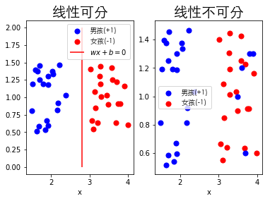
# 异常点导致数据线性不可分图例
import matplotlib.pyplot as plt
from matplotlib.font_manager import FontProperties
%matplotlib inline
font = FontProperties(fname='/Library/Fonts/Heiti.ttc')

x1 = [2, 2.5, 3.2, 6.5]
x11 = [1, 4.5, 5, 6]
x2 = [1.2, 1.4, 1.5, 1.2]
x22 = [1, 1.5, 1.3, 1]

plt.scatter(x1, x2, s=50, color='b')
plt.scatter(x11, x22, s=50, color='r')
plt.vlines(3.9, 0.8, 2, colors="g", linestyles="-",
           label='$w*x+b=0$', alpha=0.2)
plt.text(1.1, 1.1, s='异常点A', fontsize=15, color='k',
         ha='center', fontproperties=font)
plt.text(6.3, 1.3, s='异常点B', fontsize=15, color='k',
         ha='center', fontproperties=font)
plt.legend()
plt.show()

  上图可以看出由于异常点A和异常点B可能导致无法按照线性可分支持向量机对上述数据集分类。

# 异常点导致模型泛化能力变差图例
import numpy as np
import matplotlib.pyplot as plt
from matplotlib.font_manager import FontProperties
from sklearn import svm
%matplotlib inline
font = FontProperties(fname='/Library/Fonts/Heiti.ttc')

np.random.seed(8)  # 保证数据随机的唯一性

# 构造线性可分数据点
array = np.random.randn(20, 2)
X = np.r_[array-[3, 3], array+[3, 3]]
y = [0]*20+[1]*20

# 建立svm模型
clf = svm.SVC(kernel='linear')
clf.fit(X, y)

# 构造等网个方阵
x1_min, x1_max = X[:, 0].min(), X[:, 0].max(),
x2_min, x2_max = X[:, 1].min(), X[:, 1].max(),
x1, x2 = np.meshgrid(np.linspace(x1_min, x1_max),
                     np.linspace(x2_min, x2_max))

# 得到向量w: w_0x_1+w_1x_2+b=0
w = clf.coef_[0]
# 加1后才可绘制 -1 的等高线 [-1,0,1] + 1 = [0,1,2]
f = w[0]*x1 + w[1]*x2 + clf.intercept_[0] + 1

# 绘制H2，即wx+b=-1
plt.contour(x1, x2, f, [0], colors='k', linestyles='--', alpha=0.1)
plt.text(2, -4, s='$H_2={\omega}x+b=-1$', fontsize=10, color='r', ha='center')

# 绘制分隔超平面，即wx+b=0
plt.contour(x1, x2, f, [1], colors='k', alpha=0.1)
plt.text(2.5, -2, s='$\omega{x}+b=0$', fontsize=10, color='r', ha='center')
plt.text(2.5, -2.5, s='分离超平面', fontsize=10,
         color='r', ha='center', fontproperties=font)

# 绘制H1，即wx+b=1
plt.contour(x1, x2, f, [2], colors='k', linestyles='--')
plt.text(3, 0, s='$H_1=\omega{x}+b=1$', fontsize=10, color='r', ha='center')

# 绘制数据散点图
plt.scatter(X[0:20, 0], X[0:20, 1], cmap=plt.cm.Paired, marker='x')
plt.text(1, 1.8, s='支持向量', fontsize=10, color='gray',
         ha='center', fontproperties=font)

plt.scatter(X[20:40, 0], X[20:40, 1], cmap=plt.cm.Paired, marker='o')
plt.text(-1.5, -0.5, s='支持向量', fontsize=10,
         color='gray', ha='center', fontproperties=font)

# 绘制假设的异常点及假设的间隔边界，**毫无意义的代码**，为了讲解用
plt.scatter(-1.5, 3, marker='x', c='b')
plt.text(-1.5, 3.1, s='异常点A', fontsize=10,
         color='r', ha='center', fontproperties=font)
x_test = np.linspace(-3, 4, 666)
y_test = -(w[0]+0.12)*x_test - (w[1]-0.002)*x_test+clf.intercept_[0]+1.8
y_test_test = -(w[0]+0.12)*x_test - (w[1]-0.002)*x_test+clf.intercept_[0]+2.3

plt.plot(x_test, y_test, linestyle='--')
plt.plot(x_test, y_test_test)

plt.xlim(x1_min-1, x1_max+1)
plt.ylim(x2_min-1, x2_max+1)
plt.show()

  上图可以看出由于异常点导致分离超平面从淡实线变成了黄色的那条曲线，从图中可以明显看出异常点严重影响了模型的泛化能力。

  这次讲到的线性支持向量机（linear support vector machine）将修改线性可分支持向量机的硬间隔最大化为软间隔最大化解决上面有异常点导致的问题。

线性支持向量机学习目标