细分构建机器学习应用程序的流程-流程简介

1.1 sklearn安装

为了实现接下里的代码，你需要安装下列5个Python第三方库，本文只拿sklearn的安装举例，如果有同学已经安装sklearn，可以把你的sklearn更新到最新版本，其他库同理。

numpy 1.15.4
scipy 1.1.0
matplotlib 3.0.2
pandas 0.23.4
scikit-learn 0.20.1

安装方式为：

pip install sklearn

更新方式为：

pip install --upgrade sklearn

sklearn英文文档：https://scikit-learn.org/stable/index.html

sklear中文文档：http://sklearn.apachecn.org/#/

 # 终端输入，安装sklear，其他库同理
!pip install sklearn

 Requirement already satisfied: sklearn in /Applications/anaconda3/lib/python3.7/site-packages (0.0)
Requirement already satisfied: scikit-learn in /Applications/anaconda3/lib/python3.7/site-packages (from sklearn) (0.20.1)
Requirement already satisfied: numpy>=1.8.2 in /Applications/anaconda3/lib/python3.7/site-packages (from scikit-learn->sklearn) (1.15.4)
Requirement already satisfied: scipy>=0.13.3 in /Applications/anaconda3/lib/python3.7/site-packages (from scikit-learn->sklearn) (1.1.0)

 import sklearn
 
# 打印sklearn的版本
sklearn.__version__

 '0.20.1'

 # 终端输入，更新sklear
!pip install --upgrade sklearn

 Requirement already up-to-date: sklearn in /Applications/anaconda3/lib/python3.7/site-packages (0.0)
Requirement already satisfied, skipping upgrade: scikit-learn in /Applications/anaconda3/lib/python3.7/site-packages (from sklearn) (0.20.1)
Requirement already satisfied, skipping upgrade: numpy>=1.8.2 in /Applications/anaconda3/lib/python3.7/site-packages (from scikit-learn->sklearn) (1.15.4)
Requirement already satisfied, skipping upgrade: scipy>=0.13.3 in /Applications/anaconda3/lib/python3.7/site-packages (from scikit-learn->sklearn) (1.1.0)

1.2 sklearn功能模块

1.2.1 英文版本

1.2.2 中文版本

1.2.3 API统一的方法

模型	功能模块
estimator.fit(X_train, y_train)	estimator.fit(X_train, y_train)
estimator.predict(X_test)	estimator.transform(X_test)
get_params([deep])	get_params([deep])
set_params(**params)	set_params(**params)
适用于以下模型	适用于以下功能模块
Classification（分类）	Preprocessing（数据预处理）
Regression（回归）	Dimensionality Reduction（降维）
Clustering（聚类）	Feature Selection（特征选择）
–	Feature Extraction（特征提取）

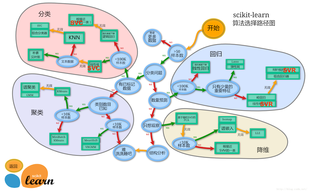
1.3 sklearn使用地图

1.3.1 英文版本

1.3.2 中文版本

1.4 构建机器学习应用程序流程

此处只是简单的带同学们了解下构建机器学习应用程序的流程，即以下6个步骤：

 1. 收集数据
2. 数据预处理
3. 训练模型
4. 测试模型
5. 优化模型
6. 持久化模型

之后会详细讲解该流程的每一个步骤。

1.4.1 收集数据

构建机器学习应用程序，无论是监督学习还是无监督学习，第一步都是获取数据，此处为了带大家对构建机器学习应用程序有一个简单的了解，所以利用sklearn自带鸢尾花数据集作展示，之后再收集数据小节会详细介绍收集数据的几种方式。

 import numpy as np
import pandas as pd
import matplotlib.pyplot as plt
from matplotlib.font_manager import FontProperties
from sklearn import datasets
%matplotlib inline
font = FontProperties(fname='/Library/Fonts/Heiti.ttc')
 
iris = datasets.load_iris()
iris

 {'data': array([[5.1, 3.5, 1.4, 0.2],
        [4.9, 3. , 1.4, 0.2],
        [4.7, 3.2, 1.3, 0.2],
        [4.6, 3.1, 1.5, 0.2],
        [5. , 3.6, 1.4, 0.2],
        [5.4, 3.9, 1.7, 0.4],
        [4.6, 3.4, 1.4, 0.3],
        [5. , 3.4, 1.5, 0.2],
        [4.4, 2.9, 1.4, 0.2],
        [4.9, 3.1, 1.5, 0.1],
        [5.4, 3.7, 1.5, 0.2],
        [4.8, 3.4, 1.6, 0.2],
        [4.8, 3. , 1.4, 0.1],
        [4.3, 3. , 1.1, 0.1],
        [5.8, 4. , 1.2, 0.2],
        [5.7, 4.4, 1.5, 0.4],
        [5.4, 3.9, 1.3, 0.4],
        [5.1, 3.5, 1.4, 0.3],
        [5.7, 3.8, 1.7, 0.3],
        [5.1, 3.8, 1.5, 0.3],
        [5.4, 3.4, 1.7, 0.2],
        [5.1, 3.7, 1.5, 0.4],
        [4.6, 3.6, 1. , 0.2],
        [5.1, 3.3, 1.7, 0.5],
        [4.8, 3.4, 1.9, 0.2],
        [5. , 3. , 1.6, 0.2],
        [5. , 3.4, 1.6, 0.4],
        [5.2, 3.5, 1.5, 0.2],
        [5.2, 3.4, 1.4, 0.2],
        [4.7, 3.2, 1.6, 0.2],
        [4.8, 3.1, 1.6, 0.2],
        [5.4, 3.4, 1.5, 0.4],
        [5.2, 4.1, 1.5, 0.1],
        [5.5, 4.2, 1.4, 0.2],
        [4.9, 3.1, 1.5, 0.2],
        [5. , 3.2, 1.2, 0.2],
        [5.5, 3.5, 1.3, 0.2],
        [4.9, 3.6, 1.4, 0.1],
        [4.4, 3. , 1.3, 0.2],
        [5.1, 3.4, 1.5, 0.2],
        [5. , 3.5, 1.3, 0.3],
        [4.5, 2.3, 1.3, 0.3],
        [4.4, 3.2, 1.3, 0.2],
        [5. , 3.5, 1.6, 0.6],
        [5.1, 3.8, 1.9, 0.4],
        [4.8, 3. , 1.4, 0.3],
        [5.1, 3.8, 1.6, 0.2],
        [4.6, 3.2, 1.4, 0.2],
        [5.3, 3.7, 1.5, 0.2],
        [5. , 3.3, 1.4, 0.2],
        [7. , 3.2, 4.7, 1.4],
        [6.4, 3.2, 4.5, 1.5],
        [6.9, 3.1, 4.9, 1.5],
        [5.5, 2.3, 4. , 1.3],
        [6.5, 2.8, 4.6, 1.5],
        [5.7, 2.8, 4.5, 1.3],
        [6.3, 3.3, 4.7, 1.6],
        [4.9, 2.4, 3.3, 1. ],
        [6.6, 2.9, 4.6, 1.3],
        [5.2, 2.7, 3.9, 1.4],
        [5. , 2. , 3.5, 1. ],
        [5.9, 3. , 4.2, 1.5],
        [6. , 2.2, 4. , 1. ],
        [6.1, 2.9, 4.7, 1.4],
        [5.6, 2.9, 3.6, 1.3],
        [6.7, 3.1, 4.4, 1.4],
        [5.6, 3. , 4.5, 1.5],
        [5.8, 2.7, 4.1, 1. ],
        [6.2, 2.2, 4.5, 1.5],
        [5.6, 2.5, 3.9, 1.1],
        [5.9, 3.2, 4.8, 1.8],
        [6.1, 2.8, 4. , 1.3],
        [6.3, 2.5, 4.9, 1.5],
        [6.1, 2.8, 4.7, 1.2],
        [6.4, 2.9, 4.3, 1.3],
        [6.6, 3. , 4.4, 1.4],
        [6.8, 2.8, 4.8, 1.4],
        [6.7, 3. , 5. , 1.7],
        [6. , 2.9, 4.5, 1.5],
        [5.7, 2.6, 3.5, 1. ],
        [5.5, 2.4, 3.8, 1.1],
        [5.5, 2.4, 3.7, 1. ],
        [5.8, 2.7, 3.9, 1.2],
        [6. , 2.7, 5.1, 1.6],
        [5.4, 3. , 4.5, 1.5],
        [6. , 3.4, 4.5, 1.6],
        [6.7, 3.1, 4.7, 1.5],
        [6.3, 2.3, 4.4, 1.3],
        [5.6, 3. , 4.1, 1.3],
        [5.5, 2.5, 4. , 1.3],
        [5.5, 2.6, 4.4, 1.2],
        [6.1, 3. , 4.6, 1.4],
        [5.8, 2.6, 4. , 1.2],
        [5. , 2.3, 3.3, 1. ],
        [5.6, 2.7, 4.2, 1.3],
        [5.7, 3. , 4.2, 1.2],
        [5.7, 2.9, 4.2, 1.3],
        [6.2, 2.9, 4.3, 1.3],
        [5.1, 2.5, 3. , 1.1],
        [5.7, 2.8, 4.1, 1.3],
        [6.3, 3.3, 6. , 2.5],
        [5.8, 2.7, 5.1, 1.9],
        [7.1, 3. , 5.9, 2.1],
        [6.3, 2.9, 5.6, 1.8],
        [6.5, 3. , 5.8, 2.2],
        [7.6, 3. , 6.6, 2.1],
        [4.9, 2.5, 4.5, 1.7],
        [7.3, 2.9, 6.3, 1.8],
        [6.7, 2.5, 5.8, 1.8],
        [7.2, 3.6, 6.1, 2.5],
        [6.5, 3.2, 5.1, 2. ],
        [6.4, 2.7, 5.3, 1.9],
        [6.8, 3. , 5.5, 2.1],
        [5.7, 2.5, 5. , 2. ],
        [5.8, 2.8, 5.1, 2.4],
        [6.4, 3.2, 5.3, 2.3],
        [6.5, 3. , 5.5, 1.8],
        [7.7, 3.8, 6.7, 2.2],
        [7.7, 2.6, 6.9, 2.3],
        [6. , 2.2, 5. , 1.5],
        [6.9, 3.2, 5.7, 2.3],
        [5.6, 2.8, 4.9, 2. ],
        [7.7, 2.8, 6.7, 2. ],
        [6.3, 2.7, 4.9, 1.8],
        [6.7, 3.3, 5.7, 2.1],
        [7.2, 3.2, 6. , 1.8],
        [6.2, 2.8, 4.8, 1.8],
        [6.1, 3. , 4.9, 1.8],
        [6.4, 2.8, 5.6, 2.1],
        [7.2, 3. , 5.8, 1.6],
        [7.4, 2.8, 6.1, 1.9],
        [7.9, 3.8, 6.4, 2. ],
        [6.4, 2.8, 5.6, 2.2],
        [6.3, 2.8, 5.1, 1.5],
        [6.1, 2.6, 5.6, 1.4],
        [7.7, 3. , 6.1, 2.3],
        [6.3, 3.4, 5.6, 2.4],
        [6.4, 3.1, 5.5, 1.8],
        [6. , 3. , 4.8, 1.8],
        [6.9, 3.1, 5.4, 2.1],
        [6.7, 3.1, 5.6, 2.4],
        [6.9, 3.1, 5.1, 2.3],
        [5.8, 2.7, 5.1, 1.9],
        [6.8, 3.2, 5.9, 2.3],
        [6.7, 3.3, 5.7, 2.5],
        [6.7, 3. , 5.2, 2.3],
        [6.3, 2.5, 5. , 1.9],
        [6.5, 3. , 5.2, 2. ],
        [6.2, 3.4, 5.4, 2.3],
        [5.9, 3. , 5.1, 1.8]]),
 'target': array([0, 0, 0, 0, 0, 0, 0, 0, 0, 0, 0, 0, 0, 0, 0, 0, 0, 0, 0, 0, 0, 0,
        0, 0, 0, 0, 0, 0, 0, 0, 0, 0, 0, 0, 0, 0, 0, 0, 0, 0, 0, 0, 0, 0,
        0, 0, 0, 0, 0, 0, 1, 1, 1, 1, 1, 1, 1, 1, 1, 1, 1, 1, 1, 1, 1, 1,
        1, 1, 1, 1, 1, 1, 1, 1, 1, 1, 1, 1, 1, 1, 1, 1, 1, 1, 1, 1, 1, 1,
        1, 1, 1, 1, 1, 1, 1, 1, 1, 1, 1, 1, 2, 2, 2, 2, 2, 2, 2, 2, 2, 2,
        2, 2, 2, 2, 2, 2, 2, 2, 2, 2, 2, 2, 2, 2, 2, 2, 2, 2, 2, 2, 2, 2,
        2, 2, 2, 2, 2, 2, 2, 2, 2, 2, 2, 2, 2, 2, 2, 2, 2, 2]),
 'target_names': array(['setosa', 'versicolor', 'virginica'], dtype='


X = iris.data
# 总共有150个样本数据，此处只打印5个
'X的个数:{}'.format(len(X)), 'X:{}'.format(X[0:5])
				
					
				
				
					
				
				
					
				
				
					
				
			
('X的个数:150',
 'X:[[5.1 3.5 1.4 0.2]\n [4.9 3.  1.4 0.2]\n [4.7 3.2 1.3 0.2]\n [4.6 3.1 1.5 0.2]\n [5.  3.6 1.4 0.2]]')
				
					
				
				
					
				
				
					
				
				
					
				
			
y = iris.target
'y的个数:{}'.format(len(y)), 'y:{}'.format(y)
				
					
				
				
					
				
				
					
				
				
					
				
			
('y的个数:150',
 'y:[0 0 0 0 0 0 0 0 0 0 0 0 0 0 0 0 0 0 0 0 0 0 0 0 0 0 0 0 0 0 0 0 0 0 0 0 0\n 0 0 0 0 0 0 0 0 0 0 0 0 0 1 1 1 1 1 1 1 1 1 1 1 1 1 1 1 1 1 1 1 1 1 1 1 1\n 1 1 1 1 1 1 1 1 1 1 1 1 1 1 1 1 1 1 1 1 1 1 1 1 1 1 2 2 2 2 2 2 2 2 2 2 2\n 2 2 2 2 2 2 2 2 2 2 2 2 2 2 2 2 2 2 2 2 2 2 2 2 2 2 2 2 2 2 2 2 2 2 2 2 2\n 2 2]')
				
					
				
				
					
				
				
					
				
				
					
				
			
# pandas可视化数据
df = pd.DataFrame(X, columns=iris.feature_names)
df['target'] = y
df.plot(figsize=(10, 8))
plt.show()
				
					
				
				
					
				
				
					
				
				
					
				
			

# matplotlib可视化
# matplotlib适合二维可视化，因此只选特征1、2，即萼片长度、萼片宽度
# 取所有行的第1，2列特征
X_ = X[:, [0, 1]]
 
# 取出山鸢尾数据
plt.scatter(X_[0:50, 0], X_[0:50, 1], color='r', label='山鸢尾', s=10)
# 取出杂色鸢尾数据
plt.scatter(X_[50:100, 0], X_[50:100, 1], color='g', label='杂色鸢尾', s=50)
# 取出维吉尼亚鸢尾
plt.scatter(X_[100:150, 0], X_[100:150, 1], color='b', label='维吉尼亚鸢尾', s=100)
 
plt.legend(prop=font)
plt.xlabel('萼片长度', fontproperties=font, fontsize=15)
plt.ylabel('萼片宽度', fontproperties=font, fontsize=15)
plt.title('萼片长度-萼片宽度', fontproperties=font, fontsize=20)
plt.show()
				
					
				
				
					
				
				
					
				
				
					
				
			

1.4.2 数据预处理
  可以发现鸢尾花数据的某一个特征的特征值最小值和最大值差距非常大，为了解决上述相同权重特征不同尺度的问题，可以使用机器学习中的最小-最大标准化做处理，把他们两个值压缩在$[0-1]$区间内。
  最小-最大标准化公式：

$$

x{norm}^{(i)}={\frac{x^{(i)}-x{min}}{x{max}-x{min}}}

$$

其中$i=1,2,\cdots,m$；$m$为样本个数；$x{min},x{max}$分别是某个的特征最小值和最大值。
from sklearn.preprocessing import MinMaxScaler
 
scaler = MinMaxScaler()
# scaler.fit_transform(X) # 等同于先fit()后transform()
scaler = scaler.fit(X)
print(X)
X1 = scaler.transform(X)
X1
				
					
				
				
					
				
				
					
				
				
					
				
			
[[5.1 3.5 1.4 0.2]
 [4.9 3.  1.4 0.2]
 [4.7 3.2 1.3 0.2]
 [4.6 3.1 1.5 0.2]
 [5.  3.6 1.4 0.2]
 [5.4 3.9 1.7 0.4]
 [4.6 3.4 1.4 0.3]
 [5.  3.4 1.5 0.2]
 [4.4 2.9 1.4 0.2]
 [4.9 3.1 1.5 0.1]
 [5.4 3.7 1.5 0.2]
 [4.8 3.4 1.6 0.2]
 [4.8 3.  1.4 0.1]
 [4.3 3.  1.1 0.1]
 [5.8 4.  1.2 0.2]
 [5.7 4.4 1.5 0.4]
 [5.4 3.9 1.3 0.4]
 [5.1 3.5 1.4 0.3]
 [5.7 3.8 1.7 0.3]
 [5.1 3.8 1.5 0.3]
 [5.4 3.4 1.7 0.2]
 [5.1 3.7 1.5 0.4]
 [4.6 3.6 1.  0.2]
 [5.1 3.3 1.7 0.5]
 [4.8 3.4 1.9 0.2]
 [5.  3.  1.6 0.2]
 [5.  3.4 1.6 0.4]
 [5.2 3.5 1.5 0.2]
 [5.2 3.4 1.4 0.2]
 [4.7 3.2 1.6 0.2]
 [4.8 3.1 1.6 0.2]
 [5.4 3.4 1.5 0.4]
 [5.2 4.1 1.5 0.1]
 [5.5 4.2 1.4 0.2]
 [4.9 3.1 1.5 0.2]
 [5.  3.2 1.2 0.2]
 [5.5 3.5 1.3 0.2]
 [4.9 3.6 1.4 0.1]
 [4.4 3.  1.3 0.2]
 [5.1 3.4 1.5 0.2]
 [5.  3.5 1.3 0.3]
 [4.5 2.3 1.3 0.3]
 [4.4 3.2 1.3 0.2]
 [5.  3.5 1.6 0.6]
 [5.1 3.8 1.9 0.4]
 [4.8 3.  1.4 0.3]
 [5.1 3.8 1.6 0.2]
 [4.6 3.2 1.4 0.2]
 [5.3 3.7 1.5 0.2]
 [5.  3.3 1.4 0.2]
 [7.  3.2 4.7 1.4]
 [6.4 3.2 4.5 1.5]
 [6.9 3.1 4.9 1.5]
 [5.5 2.3 4.  1.3]
 [6.5 2.8 4.6 1.5]
 [5.7 2.8 4.5 1.3]
 [6.3 3.3 4.7 1.6]
 [4.9 2.4 3.3 1. ]
 [6.6 2.9 4.6 1.3]
 [5.2 2.7 3.9 1.4]
 [5.  2.  3.5 1. ]
 [5.9 3.  4.2 1.5]
 [6.  2.2 4.  1. ]
 [6.1 2.9 4.7 1.4]
 [5.6 2.9 3.6 1.3]
 [6.7 3.1 4.4 1.4]
 [5.6 3.  4.5 1.5]
 [5.8 2.7 4.1 1. ]
 [6.2 2.2 4.5 1.5]
 [5.6 2.5 3.9 1.1]
 [5.9 3.2 4.8 1.8]
 [6.1 2.8 4.  1.3]
 [6.3 2.5 4.9 1.5]
 [6.1 2.8 4.7 1.2]
 [6.4 2.9 4.3 1.3]
 [6.6 3.  4.4 1.4]
 [6.8 2.8 4.8 1.4]
 [6.7 3.  5.  1.7]
 [6.  2.9 4.5 1.5]
 [5.7 2.6 3.5 1. ]
 [5.5 2.4 3.8 1.1]
 [5.5 2.4 3.7 1. ]
 [5.8 2.7 3.9 1.2]
 [6.  2.7 5.1 1.6]
 [5.4 3.  4.5 1.5]
 [6.  3.4 4.5 1.6]
 [6.7 3.1 4.7 1.5]
 [6.3 2.3 4.4 1.3]
 [5.6 3.  4.1 1.3]
 [5.5 2.5 4.  1.3]
 [5.5 2.6 4.4 1.2]
 [6.1 3.  4.6 1.4]
 [5.8 2.6 4.  1.2]
 [5.  2.3 3.3 1. ]
 [5.6 2.7 4.2 1.3]
 [5.7 3.  4.2 1.2]
 [5.7 2.9 4.2 1.3]
 [6.2 2.9 4.3 1.3]
 [5.1 2.5 3.  1.1]
 [5.7 2.8 4.1 1.3]
 [6.3 3.3 6.  2.5]
 [5.8 2.7 5.1 1.9]
 [7.1 3.  5.9 2.1]
 [6.3 2.9 5.6 1.8]
 [6.5 3.  5.8 2.2]
 [7.6 3.  6.6 2.1]
 [4.9 2.5 4.5 1.7]
 [7.3 2.9 6.3 1.8]
 [6.7 2.5 5.8 1.8]
 [7.2 3.6 6.1 2.5]
 [6.5 3.2 5.1 2. ]
 [6.4 2.7 5.3 1.9]
 [6.8 3.  5.5 2.1]
 [5.7 2.5 5.  2. ]
 [5.8 2.8 5.1 2.4]
 [6.4 3.2 5.3 2.3]
 [6.5 3.  5.5 1.8]
 [7.7 3.8 6.7 2.2]
 [7.7 2.6 6.9 2.3]
 [6.  2.2 5.  1.5]
 [6.9 3.2 5.7 2.3]
 [5.6 2.8 4.9 2. ]
 [7.7 2.8 6.7 2. ]
 [6.3 2.7 4.9 1.8]
 [6.7 3.3 5.7 2.1]
 [7.2 3.2 6.  1.8]
 [6.2 2.8 4.8 1.8]
 [6.1 3.  4.9 1.8]
 [6.4 2.8 5.6 2.1]
 [7.2 3.  5.8 1.6]
 [7.4 2.8 6.1 1.9]
 [7.9 3.8 6.4 2. ]
 [6.4 2.8 5.6 2.2]
 [6.3 2.8 5.1 1.5]
 [6.1 2.6 5.6 1.4]
 [7.7 3.  6.1 2.3]
 [6.3 3.4 5.6 2.4]
 [6.4 3.1 5.5 1.8]
 [6.  3.  4.8 1.8]
 [6.9 3.1 5.4 2.1]
 [6.7 3.1 5.6 2.4]
 [6.9 3.1 5.1 2.3]
 [5.8 2.7 5.1 1.9]
 [6.8 3.2 5.9 2.3]
 [6.7 3.3 5.7 2.5]
 [6.7 3.  5.2 2.3]
 [6.3 2.5 5.  1.9]
 [6.5 3.  5.2 2. ]
 [6.2 3.4 5.4 2.3]
 [5.9 3.  5.1 1.8]]
 
array([[0.22222222, 0.625     , 0.06779661, 0.04166667],
       [0.16666667, 0.41666667, 0.06779661, 0.04166667],
       [0.11111111, 0.5       , 0.05084746, 0.04166667],
       [0.08333333, 0.45833333, 0.08474576, 0.04166667],
       [0.19444444, 0.66666667, 0.06779661, 0.04166667],
       [0.30555556, 0.79166667, 0.11864407, 0.125     ],
       [0.08333333, 0.58333333, 0.06779661, 0.08333333],
       [0.19444444, 0.58333333, 0.08474576, 0.04166667],
       [0.02777778, 0.375     , 0.06779661, 0.04166667],
       [0.16666667, 0.45833333, 0.08474576, 0.        ],
       [0.30555556, 0.70833333, 0.08474576, 0.04166667],
       [0.13888889, 0.58333333, 0.10169492, 0.04166667],
       [0.13888889, 0.41666667, 0.06779661, 0.        ],
       [0.        , 0.41666667, 0.01694915, 0.        ],
       [0.41666667, 0.83333333, 0.03389831, 0.04166667],
       [0.38888889, 1.        , 0.08474576, 0.125     ],
       [0.30555556, 0.79166667, 0.05084746, 0.125     ],
       [0.22222222, 0.625     , 0.06779661, 0.08333333],
       [0.38888889, 0.75      , 0.11864407, 0.08333333],
       [0.22222222, 0.75      , 0.08474576, 0.08333333],
       [0.30555556, 0.58333333, 0.11864407, 0.04166667],
       [0.22222222, 0.70833333, 0.08474576, 0.125     ],
       [0.08333333, 0.66666667, 0.        , 0.04166667],
       [0.22222222, 0.54166667, 0.11864407, 0.16666667],
       [0.13888889, 0.58333333, 0.15254237, 0.04166667],
       [0.19444444, 0.41666667, 0.10169492, 0.04166667],
       [0.19444444, 0.58333333, 0.10169492, 0.125     ],
       [0.25      , 0.625     , 0.08474576, 0.04166667],
       [0.25      , 0.58333333, 0.06779661, 0.04166667],
       [0.11111111, 0.5       , 0.10169492, 0.04166667],
       [0.13888889, 0.45833333, 0.10169492, 0.04166667],
       [0.30555556, 0.58333333, 0.08474576, 0.125     ],
       [0.25      , 0.875     , 0.08474576, 0.        ],
       [0.33333333, 0.91666667, 0.06779661, 0.04166667],
       [0.16666667, 0.45833333, 0.08474576, 0.04166667],
       [0.19444444, 0.5       , 0.03389831, 0.04166667],
       [0.33333333, 0.625     , 0.05084746, 0.04166667],
       [0.16666667, 0.66666667, 0.06779661, 0.        ],
       [0.02777778, 0.41666667, 0.05084746, 0.04166667],
       [0.22222222, 0.58333333, 0.08474576, 0.04166667],
       [0.19444444, 0.625     , 0.05084746, 0.08333333],
       [0.05555556, 0.125     , 0.05084746, 0.08333333],
       [0.02777778, 0.5       , 0.05084746, 0.04166667],
       [0.19444444, 0.625     , 0.10169492, 0.20833333],
       [0.22222222, 0.75      , 0.15254237, 0.125     ],
       [0.13888889, 0.41666667, 0.06779661, 0.08333333],
       [0.22222222, 0.75      , 0.10169492, 0.04166667],
       [0.08333333, 0.5       , 0.06779661, 0.04166667],
       [0.27777778, 0.70833333, 0.08474576, 0.04166667],
       [0.19444444, 0.54166667, 0.06779661, 0.04166667],
       [0.75      , 0.5       , 0.62711864, 0.54166667],
       [0.58333333, 0.5       , 0.59322034, 0.58333333],
       [0.72222222, 0.45833333, 0.66101695, 0.58333333],
       [0.33333333, 0.125     , 0.50847458, 0.5       ],
       [0.61111111, 0.33333333, 0.61016949, 0.58333333],
       [0.38888889, 0.33333333, 0.59322034, 0.5       ],
       [0.55555556, 0.54166667, 0.62711864, 0.625     ],
       [0.16666667, 0.16666667, 0.38983051, 0.375     ],
       [0.63888889, 0.375     , 0.61016949, 0.5       ],
       [0.25      , 0.29166667, 0.49152542, 0.54166667],
       [0.19444444, 0.        , 0.42372881, 0.375     ],
       [0.44444444, 0.41666667, 0.54237288, 0.58333333],
       [0.47222222, 0.08333333, 0.50847458, 0.375     ],
       [0.5       , 0.375     , 0.62711864, 0.54166667],
       [0.36111111, 0.375     , 0.44067797, 0.5       ],
       [0.66666667, 0.45833333, 0.57627119, 0.54166667],
       [0.36111111, 0.41666667, 0.59322034, 0.58333333],
       [0.41666667, 0.29166667, 0.52542373, 0.375     ],
       [0.52777778, 0.08333333, 0.59322034, 0.58333333],
       [0.36111111, 0.20833333, 0.49152542, 0.41666667],
       [0.44444444, 0.5       , 0.6440678 , 0.70833333],
       [0.5       , 0.33333333, 0.50847458, 0.5       ],
       [0.55555556, 0.20833333, 0.66101695, 0.58333333],
       [0.5       , 0.33333333, 0.62711864, 0.45833333],
       [0.58333333, 0.375     , 0.55932203, 0.5       ],
       [0.63888889, 0.41666667, 0.57627119, 0.54166667],
       [0.69444444, 0.33333333, 0.6440678 , 0.54166667],
       [0.66666667, 0.41666667, 0.6779661 , 0.66666667],
       [0.47222222, 0.375     , 0.59322034, 0.58333333],
       [0.38888889, 0.25      , 0.42372881, 0.375     ],
       [0.33333333, 0.16666667, 0.47457627, 0.41666667],
       [0.33333333, 0.16666667, 0.45762712, 0.375     ],
       [0.41666667, 0.29166667, 0.49152542, 0.45833333],
       [0.47222222, 0.29166667, 0.69491525, 0.625     ],
       [0.30555556, 0.41666667, 0.59322034, 0.58333333],
       [0.47222222, 0.58333333, 0.59322034, 0.625     ],
       [0.66666667, 0.45833333, 0.62711864, 0.58333333],
       [0.55555556, 0.125     , 0.57627119, 0.5       ],
       [0.36111111, 0.41666667, 0.52542373, 0.5       ],
       [0.33333333, 0.20833333, 0.50847458, 0.5       ],
       [0.33333333, 0.25      , 0.57627119, 0.45833333],
       [0.5       , 0.41666667, 0.61016949, 0.54166667],
       [0.41666667, 0.25      , 0.50847458, 0.45833333],
       [0.19444444, 0.125     , 0.38983051, 0.375     ],
       [0.36111111, 0.29166667, 0.54237288, 0.5       ],
       [0.38888889, 0.41666667, 0.54237288, 0.45833333],
       [0.38888889, 0.375     , 0.54237288, 0.5       ],
       [0.52777778, 0.375     , 0.55932203, 0.5       ],
       [0.22222222, 0.20833333, 0.33898305, 0.41666667],
       [0.38888889, 0.33333333, 0.52542373, 0.5       ],
       [0.55555556, 0.54166667, 0.84745763, 1.        ],
       [0.41666667, 0.29166667, 0.69491525, 0.75      ],
       [0.77777778, 0.41666667, 0.83050847, 0.83333333],
       [0.55555556, 0.375     , 0.77966102, 0.70833333],
       [0.61111111, 0.41666667, 0.81355932, 0.875     ],
       [0.91666667, 0.41666667, 0.94915254, 0.83333333],
       [0.16666667, 0.20833333, 0.59322034, 0.66666667],
       [0.83333333, 0.375     , 0.89830508, 0.70833333],
       [0.66666667, 0.20833333, 0.81355932, 0.70833333],
       [0.80555556, 0.66666667, 0.86440678, 1.        ],
       [0.61111111, 0.5       , 0.69491525, 0.79166667],
       [0.58333333, 0.29166667, 0.72881356, 0.75      ],
       [0.69444444, 0.41666667, 0.76271186, 0.83333333],
       [0.38888889, 0.20833333, 0.6779661 , 0.79166667],
       [0.41666667, 0.33333333, 0.69491525, 0.95833333],
       [0.58333333, 0.5       , 0.72881356, 0.91666667],
       [0.61111111, 0.41666667, 0.76271186, 0.70833333],
       [0.94444444, 0.75      , 0.96610169, 0.875     ],
       [0.94444444, 0.25      , 1.        , 0.91666667],
       [0.47222222, 0.08333333, 0.6779661 , 0.58333333],
       [0.72222222, 0.5       , 0.79661017, 0.91666667],
       [0.36111111, 0.33333333, 0.66101695, 0.79166667],
       [0.94444444, 0.33333333, 0.96610169, 0.79166667],
       [0.55555556, 0.29166667, 0.66101695, 0.70833333],
       [0.66666667, 0.54166667, 0.79661017, 0.83333333],
       [0.80555556, 0.5       , 0.84745763, 0.70833333],
       [0.52777778, 0.33333333, 0.6440678 , 0.70833333],
       [0.5       , 0.41666667, 0.66101695, 0.70833333],
       [0.58333333, 0.33333333, 0.77966102, 0.83333333],
       [0.80555556, 0.41666667, 0.81355932, 0.625     ],
       [0.86111111, 0.33333333, 0.86440678, 0.75      ],
       [1.        , 0.75      , 0.91525424, 0.79166667],
       [0.58333333, 0.33333333, 0.77966102, 0.875     ],
       [0.55555556, 0.33333333, 0.69491525, 0.58333333],
       [0.5       , 0.25      , 0.77966102, 0.54166667],
       [0.94444444, 0.41666667, 0.86440678, 0.91666667],
       [0.55555556, 0.58333333, 0.77966102, 0.95833333],
       [0.58333333, 0.45833333, 0.76271186, 0.70833333],
       [0.47222222, 0.41666667, 0.6440678 , 0.70833333],
       [0.72222222, 0.45833333, 0.74576271, 0.83333333],
       [0.66666667, 0.45833333, 0.77966102, 0.95833333],
       [0.72222222, 0.45833333, 0.69491525, 0.91666667],
       [0.41666667, 0.29166667, 0.69491525, 0.75      ],
       [0.69444444, 0.5       , 0.83050847, 0.91666667],
       [0.66666667, 0.54166667, 0.79661017, 1.        ],
       [0.66666667, 0.41666667, 0.71186441, 0.91666667],
       [0.55555556, 0.20833333, 0.6779661 , 0.75      ],
       [0.61111111, 0.41666667, 0.71186441, 0.79166667],
       [0.52777778, 0.58333333, 0.74576271, 0.91666667],
       [0.44444444, 0.41666667, 0.69491525, 0.70833333]])
				
					
				
				
					
				
				
					
				
				
					
				
			
1.4.3 训练模型
  对于不同的问题需要考虑不同的机器学习算法，如分类问题使用分类算法；回归问题使用回归算法……
  对于鸢尾花分类问题，可以考虑使用分类问题，但是使用哪个分类算法呢？我们可以从sklearn使用地图中获取。
  鸢尾花的样本数大于50个->属于分类问题->有已标记数据->样本数小于100K->线性核SVD(LinearSVC)
from sklearn.model_selection import train_test_split
 
# 把训练集按照7:3的比例分成训练集和测试集
X_train, X_test, y_train, y_test = train_test_split(X, y, test_size=1/3)
'训练集长度:{}'.format(len(y_train)), '测试集长度:{}'.format(len(y_test))
				
					
				
				
					
				
				
					
				
				
					
				
			
('训练集长度:100', '测试集长度:50')
				
					
				
				
					
				
				
					
				
				
					
				
			
y_train
				
					
				
				
					
				
				
					
				
				
					
				
			
array([1, 0, 0, 0, 2, 1, 1, 0, 2, 2, 2, 0, 1, 0, 2, 1, 0, 0, 1, 2, 0, 1,
       1, 2, 0, 2, 0, 0, 2, 2, 2, 1, 0, 2, 0, 1, 2, 0, 1, 2, 1, 1, 0, 1,
       1, 0, 1, 2, 2, 2, 0, 2, 2, 1, 2, 2, 1, 2, 0, 1, 0, 2, 0, 1, 1, 1,
       0, 0, 1, 0, 2, 2, 0, 2, 0, 1, 1, 1, 1, 0, 1, 1, 2, 0, 0, 1, 1, 1,
       2, 1, 2, 0, 2, 0, 1, 0, 1, 0, 0, 2])
				
					
				
				
					
				
				
					
				
				
					
				
			
y_test
				
					
				
				
					
				
				
					
				
				
					
				
			
array([1, 2, 1, 0, 0, 2, 1, 2, 2, 1, 2, 0, 2, 0, 0, 1, 1, 1, 2, 1, 0, 2,
       0, 1, 2, 1, 2, 2, 0, 2, 2, 2, 0, 1, 2, 2, 2, 1, 2, 0, 0, 0, 1, 0,
       1, 2, 1, 0, 0, 0])
				
					
				
				
					
				
				
					
				
				
					
				
			
from sklearn.svm import SVC
# 同理
from sklearn.svm import LinearSVC
 
# probability=Ture时才能打印分类概率，即才能使用下面的predict_proba()方法
clf = SVC(kernel='linear', probability=True)
# 训练数据
clf.fit(X_train, y_train)
# 预测数据分类结果
y_prd = clf.predict(X_test)
y_prd
				
					
				
				
					
				
				
					
				
				
					
				
			
array([1, 2, 1, 0, 0, 2, 1, 2, 2, 1, 2, 0, 2, 0, 0, 1, 1, 1, 2, 1, 0, 2,
       0, 1, 2, 1, 2, 2, 0, 2, 2, 2, 0, 1, 2, 2, 2, 2, 2, 0, 0, 0, 2, 0,
       1, 2, 1, 0, 0, 0])
				
					
				
				
					
				
				
					
				
				
					
				
			
y_prd-y_test
				
					
				
				
					
				
				
					
				
				
					
				
			
array([0, 0, 0, 0, 0, 0, 0, 0, 0, 0, 0, 0, 0, 0, 0, 0, 0, 0, 0, 0, 0, 0,
       0, 0, 0, 0, 0, 0, 0, 0, 0, 0, 0, 0, 0, 0, 0, 1, 0, 0, 0, 0, 1, 0,
       0, 0, 0, 0, 0, 0])
				
					
				
				
					
				
				
					
				
				
					
				
			
clf.get_params()
				
					
				
				
					
				
				
					
				
				
					
				
			
{'C': 1.0,
 'cache_size': 200,
 'class_weight': None,
 'coef0': 0.0,
 'decision_function_shape': 'ovr',
 'degree': 3,
 'gamma': 'auto_deprecated',
 'kernel': 'linear',
 'max_iter': -1,
 'probability': True,
 'random_state': None,
 'shrinking': True,
 'tol': 0.001,
 'verbose': False}
				
					
				
				
					
				
				
					
				
				
					
				
			
clf.C
				
					
				
				
					
				
				
					
				
				
					
				
			
1.0
				
					
				
				
					
				
				
					
				
				
					
				
			
clf.set_params(C=2)
				
					
				
				
					
				
				
					
				
				
					
				
			
SVC(C=2, cache_size=200, class_weight=None, coef0=0.0,
  decision_function_shape='ovr', degree=3, gamma='auto_deprecated',
  kernel='linear', max_iter=-1, probability=True, random_state=None,
  shrinking=True, tol=0.001, verbose=False)
				
					
				
				
					
				
				
					
				
				
					
				
			
clf.get_params()
				
					
				
				
					
				
				
					
				
				
					
				
			
{'C': 2,
 'cache_size': 200,
 'class_weight': None,
 'coef0': 0.0,
 'decision_function_shape': 'ovr',
 'degree': 3,
 'gamma': 'auto_deprecated',
 'kernel': 'linear',
 'max_iter': -1,
 'probability': True,
 'random_state': None,
 'shrinking': True,
 'tol': 0.001,
 'verbose': False}
				
					
				
				
					
				
				
					
				
				
					
				
			
# 打印1-5行的所有列
clf.predict_proba(X_test)[0:5, :]
				
					
				
				
					
				
				
					
				
				
					
				
			
array([[0.02073772, 0.94985386, 0.02940841],
       [0.93450081, 0.04756914, 0.01793006],
       [0.00769491, 0.90027802, 0.09202706],
       [0.96549643, 0.02213395, 0.01236963],
       [0.01035414, 0.91467105, 0.07497481]])
				
					
				
				
					
				
				
					
				
				
					
				
			
# 查看模型得分，此处为准确率
clf.score(X_test, y_test)
				
					
				
				
					
				
				
					
				
				
					
				
			
0.96
				
					
				
				
					
				
				
					
				
				
					
				
			
1.4.4 测试模型
  测试模型则是在第二部分说的，使用模型性能度量工具测试模型的性能。上一节的score其实就是一种度量模型性能的工具，但是score只是对模型做了一个简单的评估，我们通常使用sklearn.metircs下的模块度量模型性能；使用sklearn.model_selection下的模块评估模型的泛化能力。
1.4.4.1 metircs测试模型
from sklearn.metrics import classification_report
 
print(classification_report(y, clf.predict(X), target_names=iris.target_names))
				
					
				
				
					
				
				
					
				
				
					
				
			
              precision    recall  f1-score   support
 
      setosa       1.00      1.00      1.00        50
  versicolor       1.00      0.96      0.98        50
   virginica       0.96      1.00      0.98        50
 
   micro avg       0.99      0.99      0.99       150
   macro avg       0.99      0.99      0.99       150
weighted avg       0.99      0.99      0.99       150
				
					
				
				
					
				
				
					
				
				
					
				
			
1.4.4.2 k折交叉验证
此处使用k折交叉验证度量模型性能。
  k折交叉验证：

将数据随机的分为?个子集（?的取值范围一般在[1−20]之间），然后取出?−1个子集进行训练，另一个子集用作测试模型，重复?次这个过程，得到最优模型。


将数据分为$k$个子集
选择$k-1$个子集训练模型
选择另一个子集测试模型
重复2-3步，直至有$k$个模型
对$k$个模型的预测结果取平均值

  下图为10折交叉验证示意图。
[外链图片转存失败,源站可能有防盗链机制,建议将图片保存下来直接上传(img-pTFy8dnD-1583320447319)(第四部分-10折交叉验证.jpg)]
from sklearn.model_selection import cross_val_score
 
# 10个模型的各自得分
scores = cross_val_score(clf, X, y, cv=10)
scores
				
					
				
				
					
				
				
					
				
				
					
				
			
array([1.        , 1.        , 1.        , 1.        , 0.86666667,
       1.        , 0.93333333, 1.        , 1.        , 1.        ])
				
					
				
				
					
				
				
					
				
				
					
				
			
# 平均得分和置信区间
print('准确率:{:.4f}(+/-{:.4f})'.format(scores.mean(), scores.std()*2))
				
					
				
				
					
				
				
					
				
				
					
				
			
准确率:0.9800(+/-0.0854)
				
					
				
				
					
				
				
					
				
				
					
				
			
1.4.5 优化模型
  训练并测试模型已经让我们得到了最优的参数，优化模型其实相当于找出能够使得模型性能最好的超参数，也可以理解成我们的验证集的作用，此处我们将通过网格搜索法优化模型，得到相对最好的一组超参数。
from sklearn.svm import SVC
from sklearn.model_selection import GridSearchCV
 
# 模型
svc = SVC()
 
# 超参数列表，总共会验证4*4+4=20次，'linear'是线性核，线性核超参数有一个'C'；rbf'是高斯核，高斯核有两个超参数'C'和'gamma'
param_grid = [{'C': [0.1, 1, 10, 20], 'kernel':['linear']},
              {'C': [0.1, 1, 10, 20], 'kernel':['rbf'], 'gamma':[0.1, 1, 10, 20]}]
 
# 打分函数
scoring = 'accuracy'
 
clf = GridSearchCV(estimator=svc, param_grid=param_grid,
                   scoring=scoring, cv=10)
 
clf = clf.fit(X, y)
clf.predict(X)
				
					
				
				
					
				
				
					
				
				
					
				
			
array([0, 0, 0, 0, 0, 0, 0, 0, 0, 0, 0, 0, 0, 0, 0, 0, 0, 0, 0, 0, 0, 0,
       0, 0, 0, 0, 0, 0, 0, 0, 0, 0, 0, 0, 0, 0, 0, 0, 0, 0, 0, 0, 0, 0,
       0, 0, 0, 0, 0, 0, 1, 1, 1, 1, 1, 1, 1, 1, 1, 1, 1, 1, 1, 1, 1, 1,
       1, 1, 1, 1, 2, 1, 1, 1, 1, 1, 1, 2, 1, 1, 1, 1, 1, 2, 1, 1, 1, 1,
       1, 1, 1, 1, 1, 1, 1, 1, 1, 1, 1, 1, 2, 2, 2, 2, 2, 2, 2, 2, 2, 2,
       2, 2, 2, 2, 2, 2, 2, 2, 2, 2, 2, 2, 2, 2, 2, 2, 2, 2, 2, 2, 2, 2,
       2, 2, 2, 2, 2, 2, 2, 2, 2, 2, 2, 2, 2, 2, 2, 2, 2, 2])
				
					
				
				
					
				
				
					
				
				
					
				
			
clf.get_params()
				
					
				
				
					
				
				
					
				
				
					
				
			
{'cv': 10,
 'error_score': 'raise-deprecating',
 'estimator__C': 1.0,
 'estimator__cache_size': 200,
 'estimator__class_weight': None,
 'estimator__coef0': 0.0,
 'estimator__decision_function_shape': 'ovr',
 'estimator__degree': 3,
 'estimator__gamma': 'auto_deprecated',
 'estimator__kernel': 'rbf',
 'estimator__max_iter': -1,
 'estimator__probability': False,
 'estimator__random_state': None,
 'estimator__shrinking': True,
 'estimator__tol': 0.001,
 'estimator__verbose': False,
 'estimator': SVC(C=1.0, cache_size=200, class_weight=None, coef0=0.0,
   decision_function_shape='ovr', degree=3, gamma='auto_deprecated',
   kernel='rbf', max_iter=-1, probability=False, random_state=None,
   shrinking=True, tol=0.001, verbose=False),
 'fit_params': None,
 'iid': 'warn',
 'n_jobs': None,
 'param_grid': [{'C': [0.1, 1, 10, 20], 'kernel': ['linear']},
  {'C': [0.1, 1, 10, 20], 'kernel': ['rbf'], 'gamma': [0.1, 1, 10, 20]}],
 'pre_dispatch': '2*n_jobs',
 'refit': True,
 'return_train_score': 'warn',
 'scoring': 'accuracy',
 'verbose': 0}
				
					
				
				
					
				
				
					
				
				
					
				
			
# 查看最优的一组超参数
clf.best_params_
				
					
				
				
					
				
				
					
				
				
					
				
			
{'C': 10, 'kernel': 'linear'}
				
					
				
				
					
				
				
					
				
				
					
				
			
# 查看最优超参数下模型的准确率
clf.best_score_
				
					
				
				
					
				
				
					
				
				
					
				
			
0.98
				
					
				
				
					
				
				
					
				
				
					
				
			
1.4.6 持久化模型
  使用网格搜索得到的模型的准确率有0.98，已经是比较好的一个模型了，得到这个模型之后，我们怎么样才能做到下次再使用呢？一般会通过持久化模型的方式把上述模型保存到.plk文件中，下次从.plk文件中取出直接使用即可，通常持久化的方式只有两种，一种是通过Python自带pickle库，另一种是通过sklearn库下的joblib模块。
1.4.6.1 pickle模块
import pickle
 
# 使用pickle模块把模型序列化成字符串
pkl_str = pickle.dumps(clf)
pkl_str[0:100]
				
					
				
				
					
				
				
					
				
				
					
				
			
b'\x80\x03csklearn.model_selection._search\nGridSearchCV\nq\x00)\x81q\x01}q\x02(X\x07\x00\x00\x00scoringq\x03X\x08\x00\x00\x00accuracyq\x04X\t\x00\x00\x00estimato'
				
					
				
				
					
				
				
					
				
				
					
				
			
# 使用pickel模块反序列化字符串成为模型
clf2 = pickle.loads(pkl_str)
clf2.predict(X)
				
					
				
				
					
				
				
					
				
				
					
				
			
array([0, 0, 0, 0, 0, 0, 0, 0, 0, 0, 0, 0, 0, 0, 0, 0, 0, 0, 0, 0, 0, 0,
       0, 0, 0, 0, 0, 0, 0, 0, 0, 0, 0, 0, 0, 0, 0, 0, 0, 0, 0, 0, 0, 0,
       0, 0, 0, 0, 0, 0, 1, 1, 1, 1, 1, 1, 1, 1, 1, 1, 1, 1, 1, 1, 1, 1,
       1, 1, 1, 1, 2, 1, 1, 1, 1, 1, 1, 2, 1, 1, 1, 1, 1, 2, 1, 1, 1, 1,
       1, 1, 1, 1, 1, 1, 1, 1, 1, 1, 1, 1, 2, 2, 2, 2, 2, 2, 2, 2, 2, 2,
       2, 2, 2, 2, 2, 2, 2, 2, 2, 2, 2, 2, 2, 2, 2, 2, 2, 2, 2, 2, 2, 2,
       2, 2, 2, 2, 2, 2, 2, 2, 2, 2, 2, 2, 2, 2, 2, 2, 2, 2])
				
					
				
				
					
				
				
					
				
				
					
				
			
1.4.6.2 joblib模块
from sklearn.externals import joblib
 
# 保存模型到clf.pkl文件内
joblib.dump(clf, 'clf.pkl')
# 从clf.pkl文件内加载模型
clf3 = joblib.load('clf.pkl')
clf3.predict(X)
				
					
				
				
					
				
				
					
				
				
					
				
			
array([0, 0, 0, 0, 0, 0, 0, 0, 0, 0, 0, 0, 0, 0, 0, 0, 0, 0, 0, 0, 0, 0,
       0, 0, 0, 0, 0, 0, 0, 0, 0, 0, 0, 0, 0, 0, 0, 0, 0, 0, 0, 0, 0, 0,
       0, 0, 0, 0, 0, 0, 1, 1, 1, 1, 1, 1, 1, 1, 1, 1, 1, 1, 1, 1, 1, 1,
       1, 1, 1, 1, 2, 1, 1, 1, 1, 1, 1, 2, 1, 1, 1, 1, 1, 2, 1, 1, 1, 1,
       1, 1, 1, 1, 1, 1, 1, 1, 1, 1, 1, 1, 2, 2, 2, 2, 2, 2, 2, 2, 2, 2,
       2, 2, 2, 2, 2, 2, 2, 2, 2, 2, 2, 2, 2, 2, 2, 2, 2, 2, 2, 2, 2, 2,
       2, 2, 2, 2, 2, 2, 2, 2, 2, 2, 2, 2, 2, 2, 2, 2, 2, 2])

细分构建机器学习应用程序的流程-流程简介

1.1 sklearn安装

1.2 sklearn功能模块

1.2.1 英文版本

1.2.2 中文版本

1.2.3 API统一的方法

1.3 sklearn使用地图

1.3.1 英文版本

1.3.2 中文版本

1.4 构建机器学习应用程序流程

1.4.1 收集数据

1.4.2 数据预处理

1.4.3 训练模型

1.4.4 测试模型

1.4.4.1 metircs测试模型

1.4.4.2 k折交叉验证

1.4.5 优化模型

1.4.6 持久化模型

1.4.6.1 pickle模块

1.4.6.2 joblib模块

推荐文章